连通性问题——数据结构系列教程(c++版)

梦想不会自己发光，真正闪耀的是那个为梦狂奔的你。献给知行的孩子们！（Eric.He著）

图的连通性问题，指的是判断图中顶点之间是否能通过边相互到达。根据图的类型（无向图 / 有向图），连通性的定义和解决方法有所不同。针对无向图连通性问题，常用的算法包括深度优先搜索（DFS）、广度优先搜索（BFS），以及针对有向图强连通分量的 Kosaraju 算法、Tarjan 算法。本文将详细讲解无向图、有向图连通性的实现，内容由浅入深，所有代码可直接编译运行。

图结构的实现方式：

邻接矩阵图：是一种使用「一维数组 + 二维数组」存储顶点和边数据的图结构，稠密图中常被采用；
邻接链表图：是一种使用「数组 + 链表」存储顶点和边数据的图结构，稀疏图中常被采用；

学习经典应用场景前，请根据上面的教程封装好自定义图，所有场景实例直接复用

教程目录导航

▼

连通性问题

一、基础概念

1.1 关键概念

首先要区分两类图的连通性定义：

无向图的连通性
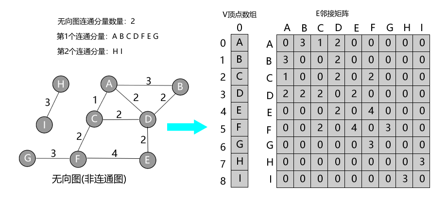
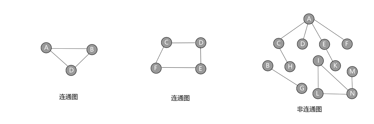
1. 连通图/非连通图：无向图中，任意两个顶点之间都存在至少一条路径，整个图是一个 “整体”。假设图中随意两点能够相互到达，则称图为连通图，否则称图为非连通图。
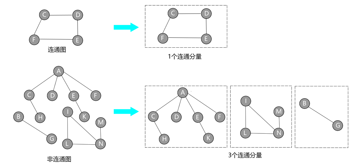
2. 连通分量：连通图的连通分量只有 1 个（自身）；若⽆向图是非连通图，但图中存在某个⼦图(最大的连通子图)符合连通图的性质，则称该⼦图为连通分量。比如一个无向图被拆成 3 个互不连通的部分，就有 3 个连通分量；
有向图的连通性
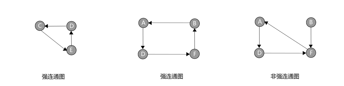
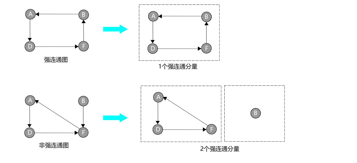
1. 强连通图/非强连通图：有向图中，任意两个顶点 u 和 v，既存在 u→v 的路径，也存在 v→u 的路径，则称图为强连通图，否则称图为非强连通图。
2. 强连通分量：若整个有向图 G 是强连通图（任意两点互相可达），则图 G 的强连通分量只有1个。若有向图非强连通，则其可以被划分为多个互不相交的强连通分量，这些分量覆盖图的所有顶点。

1.2 算法对比与选择

算法	时间复杂度	空间复杂度	适用场景
DFS/BFS遍历	O(V+E)	O(V)	无向图连通分量统计
Kosaraju 算法	O(V+E)	O(V+E)	有向图强连通分量（实现简单）
Tarjan 算法	O(V+E)	O(V)	有向图强连通分量（一次 DFS）

一、无向图连通性---DFS/BFS遍历法

从任意顶点出发，通过 DFS 或 BFS 遍历所有可达顶点。若遍历后所有顶点都被访问，则图是连通的；否则统计连通分量数。

算法解析：

初始化一个 visited 数组，标记顶点是否被访问。
遍历所有顶点，若当前顶点未被访问，则启动一次 DFS/BFS，遍历所有可达顶点。
每启动一次遍历，连通分量数加 1。


#include <iostream>
#include <vector>
#include"ArrayGraph.h"

using namespace std;

//深度优先遍历
void dfsConnect(int index, ArrayGraph& graph, bool visited[], vector<int>& component) {
    visited[index] = true;
    component.push_back(index);  // 加入当前连通分量

    // 遍历所有邻接顶点
    for (int j = 0; j < graph.vertexNum; j++) {
        // 存在边且未访问
        if (graph.graph[index][j] > NO_EDGE && !visited[j]) {
            dfsConnect(j, graph, visited, component);
        }
    }
}

//广度优先遍历
void bfsConnect(int index, ArrayGraph& graph, bool visited[], vector<int>& component) {
    int queue[MAX_VERTEX]; // 简单队列（数组实现）
    int front = 0, rear = 0; // 队列头尾指针

    // 起始顶点入队并标记访问
    visited[index] = true;
    queue[rear++] = index;

    // 队列不为空时循环
    while (front < rear) {
        // 出队并打印
        int currIndex = queue[front++];
        component.push_back(currIndex);  // 加入当前连通分量

        // 遍历所有邻接顶点
        for (int j = 0; j < graph.vertexNum; j++) {
            if (graph.graph[currIndex][j] > NO_EDGE && !visited[j]) {
                visited[j] = true;
                queue[rear++] = j;
            }
        }
    }
}

// 计算连通分量数
void countConnect(ArrayGraph& graph, vector<vector<int>>& components) {
    bool visited[MAX_VERTEX] = {false};
    int count = 0;

    for (int i = 0; i < graph.vertexNum; ++i) {
        if (!visited[i]) {
            vector<int< component;
            bfsConnect(i, graph, visited, component);
            components.push_back(component);
        }
    }
}


// 测试案例
int main() {
    ArrayGraph graph;

    // 1. 添加顶点（A、B、C、D、E、F、G、H、I）
    graph.addVertex('A');
    graph.addVertex('B');
    graph.addVertex('C');
    graph.addVertex('D');
    graph.addVertex('E');
    graph.addVertex('F');
    graph.addVertex('G');
    graph.addVertex('H');
    graph.addVertex('I');

    // 2. 添加边（有权无向图）
    graph.addEdge('A','B',3);
    graph.addEdge('A','C',1);
    graph.addEdge('A','D',2);

    graph.addEdge('B','A',3);
    graph.addEdge('B','D',2);

    graph.addEdge('C','A',1);
    graph.addEdge('C','D',2);
    graph.addEdge('C','F',2);

    graph.addEdge('D','A',2);
    graph.addEdge('D','B',2);
    graph.addEdge('D','C',2);
    graph.addEdge('D','E',2);

    graph.addEdge('E','D',2);
    graph.addEdge('E','F',4);

    graph.addEdge('F','C',2);
    graph.addEdge('F','E',4);
    graph.addEdge('F','G',3);

    graph.addEdge('G','F',3);

    graph.addEdge('H','I',3);
    graph.addEdge('I','H',3);

    // 3. 打印邻接矩阵
    graph.printAdjacency();

    // 4. 统计连通分量
    vector<vector<int>> components;
    countConnect(graph, components);

    // 5. 输出结果
    cout << "无向图连通分量数量：" << components.size() << endl;
    cout << "连通分量详情：" << endl;
    for (int i = 0; i < components.size(); ++i) {
        cout << "第" << i+1 << "个连通分量：";
        for (int node : components[i]) {
            cout << graph.vertices[node] << " ";
        }
        cout << endl;
    }

    return 0;
}

输出结果


   ===== 带权邻接矩阵 =====
     A  B  C  D  E  F  G  H  I
  A  0  3  1  2  0  0  0  0  0
  B  3  0  0  2  0  0  0  0  0
  C  1  0  0  2  0  2  0  0  0
  D  2  2  2  0  2  0  0  0  0
  E  0  0  0  2  0  4  0  0  0
  F  0  0  2  0  4  0  3  0  0
  G  0  0  0  0  0  3  0  0  0
  H  0  0  0  0  0  0  0  0  3
  I  0  0  0  0  0  0  0  3  0
========================
无向图连通分量数量：2
连通分量详情：
第1个连通分量：A B C D F E G
第2个连通分量：H I

三、有向图连通性---Kosaraju 算法

通过两次 DFS 实现强连通分量的查找。

算法解析：

对原图进行 DFS，记录顶点的后序遍历顺序，并按后序时间从晚到早排序。
将原图的所有边反向，得到逆图。
按照第一步得到的顺序，对逆图进行 DFS，每一次遍历得到的顶点集合就是一个强连通分量。


#include <iostream>
#include <vector>
#include <stack>
#include"ArrayGraph.h"

using namespace std;

stack<int> order;           // 存储后序遍历顺序

//原图的DFS，记录后序顺序
void dfsConnect1(int index, ArrayGraph& graph, bool visited[]) {
    visited[index] = true;

    // 遍历所有邻接顶点
    for (int j = 0; j < graph.vertexNum; j++) {
        // 存在边且未访问
        if (graph.graph[index][j] > NO_EDGE && !visited[j]) {
            dfsConnect1(j, graph, visited);
        }
    }
    order.push(index); // 后序入栈
}

//逆图的DFS，获取强连通分量
void dfsConnect2(int index, ArrayGraph& graph, bool visited[], vector<int>& component) {
    visited[index] = true;
    component.push_back(index);  // 加入当前连通分量

    // 遍历所有邻接顶点
    for (int j = 0; j < graph.vertexNum; j++) {
        // 存在边且未访问
        if (graph.graph[index][j] > NO_EDGE && !visited[j]) {
            dfsConnect2(j, graph, visited, component);
        }
    }
}

// 计算强连通分量数
void countKosarajuConnect(ArrayGraph& graph, ArrayGraph& graphContrary, vector<vector<int>>& components) {
    bool visited[MAX_VERTEX] = {false};

    // 步骤1：遍历原图，记录后序顺序
    for (int i = 0; i < graph.vertexNum; ++i) {
        if (!visited[i]) {
            dfsConnect1(i, graph, visited);
        }
    }

    memset(visited, false, MAX_VERTEX);// 重置访问标记

     // 步骤2：按逆序遍历逆图
     while (!order.empty()) {
         int u = order.top();
         order.pop();
         if (!visited[u]) {
             vector<int> component;
             dfsConnect2(u, graphContrary, visited, component);
             components.push_back(component);
         }
     }
}


// 测试案例
int main() {
    ArrayGraph graph;//原图
    ArrayGraph graphContrary;//逆图

    // 1. 添加顶点（A、B、C、D、E、F、G、H、I）
    graph.addVertex('A');graphContrary.addVertex('A');
    graph.addVertex('B');graphContrary.addVertex('B');
    graph.addVertex('C');graphContrary.addVertex('C');
    graph.addVertex('D');graphContrary.addVertex('D');
    graph.addVertex('E');graphContrary.addVertex('E');
    graph.addVertex('F');graphContrary.addVertex('F');
    graph.addVertex('G');graphContrary.addVertex('G');
    graph.addVertex('H');graphContrary.addVertex('H');
    graph.addVertex('I');graphContrary.addVertex('I');

    // 2. 添加边（有权有向图）
    graph.addDirectedEdge('A','B',3);graphContrary.addDirectedEdge('A','B',3);
    graph.addDirectedEdge('A','C',1);graphContrary.addDirectedEdge('A','C',1);
    graph.addDirectedEdge('A','D',2);graphContrary.addDirectedEdge('A','D',2);

    graph.addDirectedEdge('B','A',3);graphContrary.addDirectedEdge('B','A',3);
    graph.addDirectedEdge('B','D',2);graphContrary.addDirectedEdge('B','D',2);

    graph.addDirectedEdge('C','A',1);graphContrary.addDirectedEdge('C','A',1);
    graph.addDirectedEdge('C','D',2);graphContrary.addDirectedEdge('C','D',2);
    graph.addDirectedEdge('C','F',2);graphContrary.addDirectedEdge('C','F',2);

    graph.addDirectedEdge('D','A',2);graphContrary.addDirectedEdge('D','A',2);
    graph.addDirectedEdge('D','B',2);graphContrary.addDirectedEdge('D','B',2);
    graph.addDirectedEdge('D','C',2);graphContrary.addDirectedEdge('D','C',2);
    graph.addDirectedEdge('D','E',2);graphContrary.addDirectedEdge('D','E',2);

    graph.addDirectedEdge('E','D',2);graphContrary.addDirectedEdge('E','D',2);
    graph.addDirectedEdge('E','F',4);graphContrary.addDirectedEdge('E','F',4);

    graph.addDirectedEdge('F','C',2);graphContrary.addDirectedEdge('F','C',2);
    graph.addDirectedEdge('F','E',4);graphContrary.addDirectedEdge('F','E',4);
    graph.addDirectedEdge('F','G',3);graphContrary.addDirectedEdge('F','G',3);

    graph.addDirectedEdge('G','F',3);graphContrary.addDirectedEdge('G','F',3);

    graph.addDirectedEdge('H','I',3);graphContrary.addDirectedEdge('H','I',3);
    graph.addDirectedEdge('I','H',3);graphContrary.addDirectedEdge('I','H',3);

    // 3. 打印邻接矩阵
    graph.printAdjacency();

    // 4. 统计强连通分量
    vector<vector<int>> components;
    countKosarajuConnect(graph, graphContrary, components);

    // 5. 输出结果
    cout << "有向图强连通分量数量：" << components.size() << endl;
    cout << "强连通分量详情：" << endl;
    for (int i = 0; i < components.size(); ++i) {
        cout << "第" << i+1 << "个强连通分量：";
        for (int node : components[i]) {
            cout << graph.vertices[node] << " ";
        }
        cout << endl;
    }

    return 0;
}

输出结果


========= 带权邻接矩阵 ========
     A  B  C  D  E  F  G  H  I
  A  0  3  1  2  0  0  0  0  0
  B  3  0  0  2  0  0  0  0  0
  C  1  0  0  2  0  2  0  0  0
  D  2  2  2  0  2  0  0  0  0
  E  0  0  0  2  0  4  0  0  0
  F  0  0  2  0  4  0  3  0  0
  G  0  0  0  0  0  3  0  0  0
  H  0  0  0  0  0  0  0  0  3
  I  0  0  0  0  0  0  0  3  0
==============================
有向图强连通分量数量：2
强连通分量详情：
第1个强连通分量：H I
第2个强连通分量：A B D C F E G

四、有向图连通性---Tarjan 算法

Tarjan 算法是基于对图的 DFS 算法的优化，每个强连通分量为搜索树中的一棵子树。基于一次 DFS，利用时间戳和追溯值（low 值）查找强连通分量，效率更高（线性时间复杂度）。

算法解析：

dfn[u]：顶点 u 的首次访问时间戳。
low[u]：顶点 u 能够到达的最早时间戳的顶点。
栈：存储当前遍历路径上的顶点。
判断条件：当 dfn[u] == low[u] 时，栈中从栈顶到 u 的所有顶点构成一个强连通分量。


#include <iostream>
#include <vector>
#include <stack>
#include"ArrayGraph.h"

using namespace std;

int timeStamp=0;
vector<int> dfn(MAX_VERTEX,0);// 时间戳
vector<int> low(MAX_VERTEX,0);// 追溯值
vector<bool> inStack(MAX_VERTEX,false);
stack<int> st;// 存储该连通子图中的所有点。

// Tarjan 递归函数
void tarjan(int u, ArrayGraph& graph, vector<vector<int>>& components) {
   dfn[u] = low[u] = ++timeStamp; // 初始化节点 u 的时间戳与追溯值
   st.push(u);
   inStack[u] = true;
   for (int v = 0; v < graph.vertexNum; ++v) {
       if(graph.graph[u][v] != NO_EDGE)
       {
           if (!dfn[v]) { // v未被访问
               tarjan(v, graph, components);// / 递归搜索以 u 为跟的子树
               low[u] = min(low[u], low[v]);
           } else if (inStack[v]) { // v在栈中（属于当前路径）
               low[u] = min(low[u], dfn[v]);
           }
       }
   }
   // 找到强连通分量的根
   if (dfn[u] == low[u]) {
       vector<int> component;
       while (true) {
           int top = st.top();
           st.pop();
           inStack[top] = false;
           component.push_back(top);
           if (top == u) break;
       }
       components.push_back(component);
    }
}

// 计算强连通分量数
void countTarjanConnect(ArrayGraph& graph, vector<vector<int>>& components)
{
    for (int i = 0; i < graph.vertexNum; ++i) {
        if (!dfn[i]) {
            tarjan(i, graph, components);
        }
    }
}


// 测试案例
int main() {
    ArrayGraph graph;

    // 1. 添加顶点（A、B、C、D、E、F、G、H、I）
    graph.addVertex('A');
    graph.addVertex('B');
    graph.addVertex('C');
    graph.addVertex('D');
    graph.addVertex('E');
    graph.addVertex('F');
    graph.addVertex('G');
    graph.addVertex('H');
    graph.addVertex('I');

    // 2. 添加边（有权有向图）
    graph.addDirectedEdge('A','B',3);
    graph.addDirectedEdge('A','C',1);
    graph.addDirectedEdge('A','D',2);

    graph.addDirectedEdge('B','A',3);
    graph.addDirectedEdge('B','D',2);

    graph.addDirectedEdge('C','A',1);
    graph.addDirectedEdge('C','D',2);
    graph.addDirectedEdge('C','F',2);

    graph.addDirectedEdge('D','A',2);
    graph.addDirectedEdge('D','B',2);
    graph.addDirectedEdge('D','C',2);
    graph.addDirectedEdge('D','E',2);

    graph.addDirectedEdge('E','D',2);
    graph.addDirectedEdge('E','F',4);

    graph.addDirectedEdge('F','C',2);
    graph.addDirectedEdge('F','E',4);
    graph.addDirectedEdge('F','G',3);

    graph.addDirectedEdge('G','F',3);

    graph.addDirectedEdge('H','I',3);
    graph.addDirectedEdge('I','H',3);

    // 3. 打印邻接矩阵
    graph.printAdjacency();

    // 4. 统计强连通分量
    vector<vector<int>> components;
    countTarjanConnect(graph, components);

    // 5. 输出结果
    cout << "有向图强连通分量数量：" << components.size() << endl;
    cout << "强连通分量详情：" << endl;
    for (int i = 0; i < components.size(); ++i) {
        cout << "第" << i+1 << "个强连通分量：";
        for (int node : components[i]) {
            cout << graph.vertices[node] << " ";
        }
        cout << endl;
    }

    return 0;
}

输出结果


========== 带权邻接矩阵 =======
     A  B  C  D  E  F  G  H  I
  A  0  3  1  2  0  0  0  0  0
  B  3  0  0  2  0  0  0  0  0
  C  1  0  0  2  0  2  0  0  0
  D  2  2  2  0  2  0  0  0  0
  E  0  0  0  2  0  4  0  0  0
  F  0  0  2  0  4  0  3  0  0
  G  0  0  0  0  0  3  0  0  0
  H  0  0  0  0  0  0  0  0  3
  I  0  0  0  0  0  0  0  3  0
==============================
有向图强连通分量数量：2
强连通分量详情：
第1个强连通分量：G E F C D B A
第2个强连通分量：I H

返回顶部